Getting started with post-quantum cryptography: the ML-KEM key exchange

In this article, I invite you to discover the wonderful world of post-quantum cryptography with the Module-Lattice-Based Key-Encapsulation Mechanism (ML-KEM) key exchange algorithm, also known as Kyber and standardized in August 2024. The principle is to provide a way to exchange encryption keys while being robust against future quantum computers, theoretically capable of breaking some major currently used cryptographic algorithms.

Introduction

Cryptography is ubiquitous for securing our data. Thanks to it, we can guarantee essential data properties such as confidentiality, integrity, authenticity, and non-repudiation. To achieve so, it relies on mathematical problems that are difficult for an attacker to solve. However, these properties are now threatened by the future and probable arrival of the quantum computer. By using properties of the laws of quantum physics, which many perceive as magic (and they are not entirely wrong!), computing capabilities are very much upgraded compared to a classic computer. The main mathematical problems threatened by quantum computers are the discrete logarithm problem and the factorization problem, which are notably used in encryption key exchange and asymmetric encryption (using a public key to encrypt data and a private key to decrypt data).

For several years, a standardization process has aimed to provide a set of cryptographic algorithms robust to quantum computers: this is called post-quantum cryptography (sometimes also quantum-safe/proof/resistant cryptography). Among these algorithms, Module-Lattice-Based Key-Encapsulation Mechanism (ML-KEM) allows for the exchange of encryption keys. It is a post-quantum Key Encapsulation Mechanism (KEM). We will come back to this.

Post-quantum cryptography thus scares many people due to its title, which might suggest that in addition to mathematical skills, it is necessary to master quantum physics skills to understand this field. Ultimately, it remains just mathematics (and that’s already something!).
Although the quantum computer is in the proof-of-concept stage and has not yet been demonstrated to be capable of breaking traditional cryptographic algorithms historically considered robust, the National Institute of Standards and Technology (NIST) recommends eliminating the use of post-quantum vulnerable cryptography by 2035, and nearly a third of Web traffic would already be using post-quantum cryptography (according to Cloudflare). You can also check here if your Web browser supports post-quantum cryptography.

With this article, I want to answer the following questions for which I have been seeking answers in recent months:

• What is a quantum computer?
• Why does the quantum computer threaten current cryptography?
• How does post-quantum cryptography differ from current cryptography?
• How can post-quantum cryptography protect itself from quantum computers?

First, I propose to understand what a quantum computer is, then to delve into the mathematical concepts that allow us to understand the ML-KEM algorithm, which we will then see in more detail.

The post-quantum era

Richard Feynman, an American physicist, said: If you think you understand quantum mechanics, you don’t understand quantum mechanics. So don’t worry, it’s perfectly expected not to understand everything in this section!

Quantum physics

Quantum physics, born at the beginning of the 20th century, is the set of theories that describe the behavior of matter and energy at an extremely small scale, the subatomic scale (smaller than the atom). It is the branch of physics that studies the infinitely small, as opposed to classical physics such as relativity theory, which describes spacetime or gravity. The term quantum comes from the Latin “quantum” meaning “how much” or “of what amount”, which refers to the fact that at the very small scale, “grains” exist as basic components to build matter, like Legos.
Quantum physics, whose laws are those of quantum mechanics, is difficult for our brains to grasp, as the phenomena are so counter-intuitive. Here are the main ones:

• Quantization: certain observed values can only take discrete values (a finite set of values) and not continuous ones. For example, an atom has a certain number of possible energy levels, much like suddenly going from 0 to 50 km/h with your car, rather than continuously increasing the speed.
• Wave-particle duality: the concepts of wave (propagation of a disturbance in a medium) and particle are part of the same phenomenon. A good example is light composed of photons: both wave and particle.
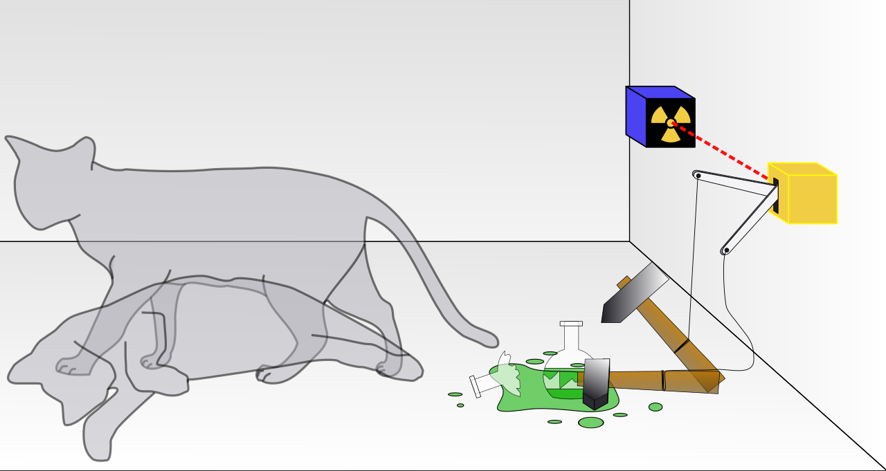
• Superposition: a particle can exist in multiple states or positions at once until a measurement is performed. This is the idea of the famous “Schrödinger’s cat” which is both dead and alive. This can be compared to tossing a coin that spins in the air before landing on heads or tails: as long as the coin is in the air, both values are possible, until the coin lands and you can read the value of heads or tails.
• Entanglement: the state of one particle can determine the one of another, regardless of the distance separating them, even light-years away (the distance light travels in one year). This is totally counter-intuitive when we know that Einstein demonstrated that there is a maximum speed for matter to travel: that of light.

Quantum computer

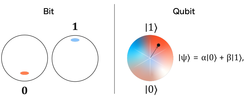
Classical computers operate on bits whose value can be 0 or 1. Quantum computers operate on quantum bits or qubits, whose value can be 0 and 1 simultaneously. This is related to the property of quantum superposition we just saw. Typically, the state of a qubit is described as follows: $$|\psi\rangle = \alpha|0\rangle + \beta|1\rangle$$ where $\alpha$ and $\beta$ are probability amplitudes, which are complex numbers (an extension of real numbers with a part containing an imaginary number $i$ such that $i^2 = -1$). The integration of complex numbers introduces the notion of phase: a kind of angle in the complex space that describes the state of the qubit.
The notation $|\psi\rangle$ means that we can observe the state of a qubit as 0 with a probability of $|\alpha|^2$ and as 1 with a probability of $|\beta|^2$. Thus $|\alpha|^2 + |\beta|^2 = 1$.

Multiple qubits can be entangled, and the state of 2 qubits can be represented as a Bell state: $$|\Phi^+\rangle = \frac{1}{\sqrt{2}}(|00\rangle + |11\rangle)$$ Therefore, the measurement of the first qubit leads to the same measurement of the other qubit.

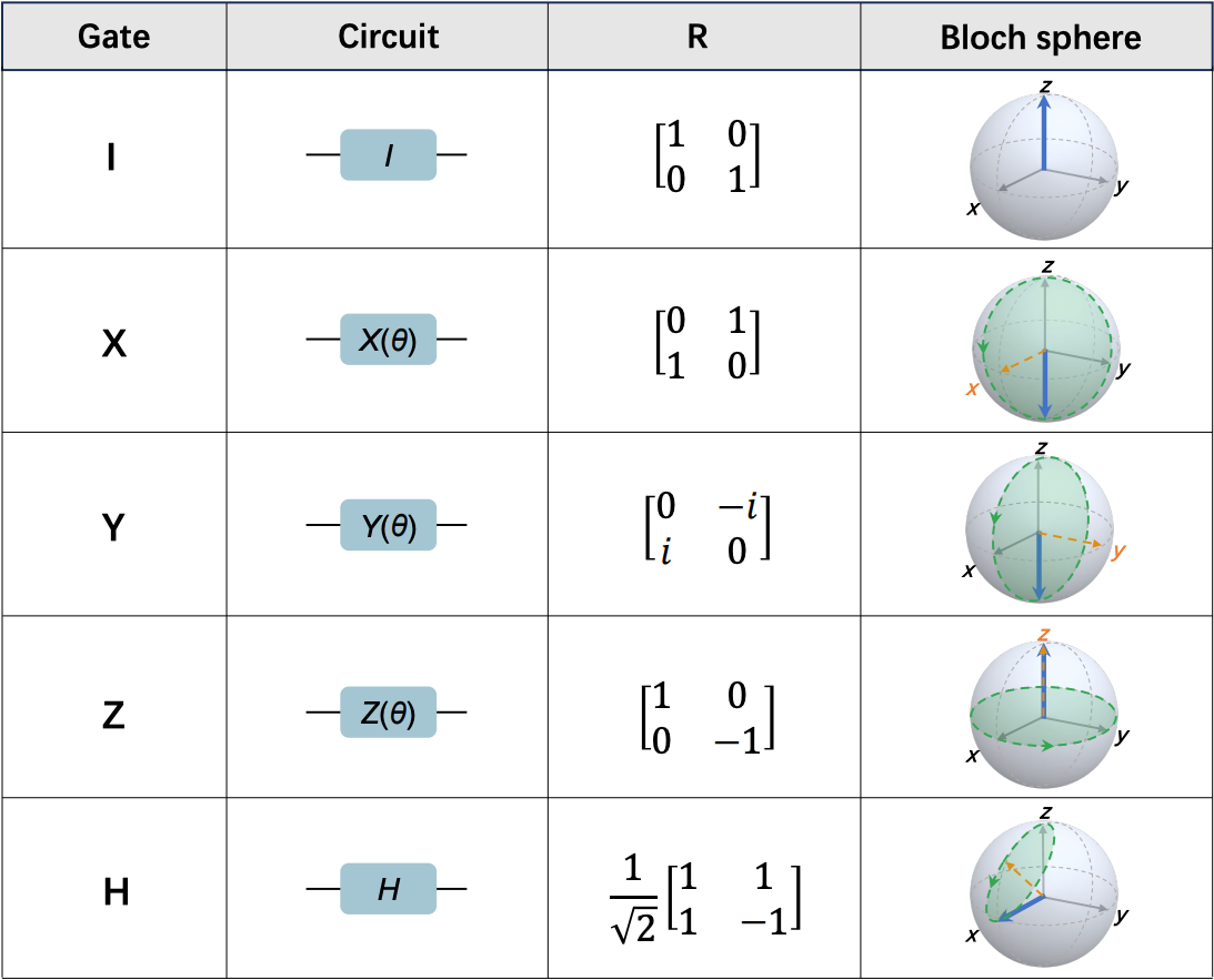
Operations on qubits within a quantum computer are performed with quantum gates. They act as groups of amplitudes, similar to how a matrix acts when multiplied by a vector. Quantum computers offer bigger computing power, because with $n$ qubits, they can process $2^n$ numbers (the amplitude of the qubits) at once, and not just $n$ numbers at once like classical computers. The role of quantum gates is to modify the probability amplitudes of the superposed states. These gates can create and manipulate superposition, as well as create entanglement between qubits, which is crucial for exploring many computational paths in parallel. Among the multiple quantum gates, some examples include:

• The Identity gate (I): keeps the qubit in the same state (for tests, synchronization, etc.).
• The Hadamard gate (H): allows creating a superposition state of two states on a qubit, enabling parallelism in calculations.
• The Pauli gates (X, Y, Z): the equivalent of classical logic gates (AND, OR, NOT…) allowing state change (X gate), phase change (Z gate), or both (Y gate).
• The Controlled-NOT gate (CNOT or CX): allows creating an entanglement state for two qubits.
• The Swap gate (S): allows swapping two qubits.

Quantum algorithms are therefore circuits of quantum gates that transform amplitudes before a final measurement of the qubits. It is this process that allows quantum computing to solve certain problems much faster than classical computers.
If I were to give you an analogy, the quantum computer is to information representation and manipulation in a computer what multithreading (parallelism of computer instructions) is to calculation within a processor.

Threats to cryptography

With this new post-quantum era, existing cryptographic algorithms are at risk. Indeed, the strength of certain mathematical problems lies in the inability of a classical computer to solve them. With quantum computing, new quantum algorithms arise, and the two most famous are Grover and Shor.

Grover’s algorithm facilitates brute-force attacks by allowing exhaustive search for solutions in a set of elements. For example, it makes it easier to find an Advanced Encryption Standard (AES) encryption key of type AES-128 among the $2^{128}$ possible keys by performing $2^{64}$ operations instead of the $2^{128}$ that a classical computer would perform. It is considered that keys longer than 200 bits, such as AES-256, offer resistance to quantum algorithms like Grover, by guaranteeing a 100-bit security margin against exhaustive search.

Shor’s algorithm allows factoring a large number into prime numbers. This is made possible by the ability to find a period in a periodic function, which allows the quantum computer to evaluate the function simultaneously for a very large number of input points, and then use a phenomenon of quantum interference (similar to a “wave” that highlights repetition) to extract this period exponentially faster than any known classical algorithm.

Rivest–Shamir–Adleman (RSA, used for digital signatures or encryption key exchange) relies precisely on the problem of factoring large prime numbers: finding $p$ and $q$ prime numbers by knowing $N$ such that $N = p \times q$. The Diffie-Hellman (DH) algorithm and its application in Elliptic Curve Cryptography (ECC) rely on the Discrete Logarithm Problem (DLP), which consists, if a value $A$ is known, in finding a value $a$ such that $A = g^a\bmod{p}$ (raising $g$ to the power $a$ is called exponentiation), with $g$ a given number and $p$ a very large prime number. However, Shor’s algorithm has demonstrated that it can reduce these problems to a period-finding problem. It transforms the difficult factorization or discrete logarithm problem into an instance of a period-finding problem in a specially constructed function.

It is therefore crucial to anticipate the research and standardization of solutions to replace algorithms like RSA, DH, or ECC.

Post-quantum cryptography

In 2016, NIST launched a call for proposals and a process to standardize post-quantum cryptographic algorithms. As a result, four algorithms have been standardized, including two for digital signatures:

• Module-Lattice-based Digital Signature Standard (ML-DSA) derived from the CRYSTALS-Dilithium algorithm;
• Stateless Hash-based Digital Signature Standard (SLH-DSA) derived from the SPHINCS+ algorithm.

and two for encryption key exchange using Key Encapsulation Mechanism (KEM):

• Module-Lattice-based Key-Encapsulation Mechanism (ML-KEM) derived from the Kyber algorithm;
• Hamming Quasi-Cyclic (HQC).

Post-quantum cryptography relies on several types of post-quantum algorithms: (error-correcting) code-based, lattice-based (which we will see right after), hash-based, or multivariate (based on polynomials with multiple variables).
I propose to dive into ML-KEM, which relies on lattices and the mathematical problem of Module Learning With Errors (MLWE).

Mathematical concepts Used in ML-KEM

To understand ML-KEM, it is interesting to understand the mathematical concepts manipulated in ML-KEM. If you really hate math, you may always skip to the next section that discusses ML-KEM, but you will have a partial understanding. If you like math a bit, it continues here!

Lattices

Let’s start with lattices. A lattice is a discrete subgroup of a Euclidean vector space. The latter is denoted $\mathbb{R}^n$, with $\mathbb{R}$ being the set of real numbers, i.e., numbers that can be represented in integer and decimal form, and $n$ the dimension of the space, i.e., the number of coordinates needed to represent points in this space (we can visually represent a space up to the 3rd dimension, when $n$ is 3). In other words, a lattice is a set of points regularly arranged in a multi-dimensional space, following a repeating pattern. With a dimension of 2 ($n=2$), a lattice is a kind of grid containing points as shown in the following figure.

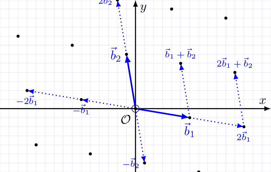
A lattice has an origin which can be seen as a kind of “starting point in the grid” allowing the lattice to be generated. We also distinguish the basis, a set of vectors that allow generating the other points and which can be seen as the “movement rules” in the grid.

In these lattices (especially in high dimensions), there are very difficult computational problems to solve (even with quantum computers), such as the Shortest Vector Problem (SVP), which consists of finding the closests point to the basis. We can also cite the Closest Vector Problem (CVP), which aims at finding the closest point to a given point. The difficulty in solving these problems is due to the immense number of possibilities existing in a high-dimensional space ($n$ being very large). Therefore, the complexity of SVP and CVP is exponential.

LWE and MLWE

Learning With Errors (LWE) consists of finding a secret vector $s$ in a vector space $\mathbb{Z}^n_q$ (the set of all $n$-dimensional vectors whose components are integers modulo $q$) of $n$ numbers given $(A, b)$ such that $b = A \cdot s + e\bmod{q}$, with $A$ being a random matrix, $e$ a random vector, and $q$ a prime number. Solving LWE is somehow equivalent to solving a specific instance of CVP on a very particular lattice. The core of LWE lies in the addition of noise (the error vector $e$) which then becomes very complex compared to a system without this noise.

A variant of LWE is *Module LWE (MLWE). MLWE operates on elements of modules over a ring. Let’s define what a ring and a module are.

A ring is an algebraic structure (a set and possible operations within that set satisfying certain properties) containing a set and two binary operations: addition and multiplication, except that here addition and multiplication are not necessarily commutative, meaning that the order of the operands can change the result of the operation. Rings can be varied: ring of integers, ring of polynomials with real coefficients, ring of polynomials whose coefficients are subject to a modulo… A polynomial is a mathematical expression formed by products and sums of constants and variables.
A module is a vector space (a set of vectors that can be added to each other or multiplied by a scalar, which is a quantity like a number that allows changing scale) where elements can be multiplied by scalars that come from a ring.

Thus, while LWE operates on vectors and matrices of integers, MLWE operates on vectors and matrices of polynomials rather than integers.

The essence and strength of ML-KEM lies in MLWE. Let’s now see how ML-KEM works.

ML-KEM

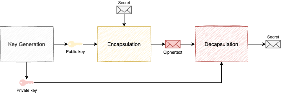
ML-KEM, called CRYSTALS-Kyber before its standardization by NIST, is a post-quantum Key Encapsulation Mechanism (KEM) based on MLWE. A KEM is an asymmetric cryptography mechanism allowing a secret to be generated and securely transmitted using a private-public key pair. It consists of three steps:

• Key generation: a public key and a private key are generated;
• Encapsulation: a secret is generated and encrypted with the public key to produce a ciphertext;
• Decapsulation: the ciphertext is decrypted with the private key to recover the original secret.

ML-KEM uses the polynomial ring $R_q = \mathbb{Z}_q[X]/(X^n + 1)$, where:

• $X^n + 1$ is the polynomial modulus: it is a polynomial whose coefficients come from $\mathbb{Z}_q$ (the set of integers modulo $q$) and which serves as the modulus in ML-KEM for operations on the polynomials themselves.
• $n$, fixed at $256$, is the degree of the polynomial $X^n + 1$ whose coefficients come from $\mathbb{Z}_q$ (the set of integers modulo $q$), $n$ is therefore by extension the dimension of the polynomials in the ring $R_q$.
• $q$, a prime number fixed at $3389$, is a prime number that is the modulus for operations on the coefficients of each polynomial.

It is within the $R_q$ workspace that ML-KEM operations take place.
Another parameter, $k$, is the dimension of the polynomial vectors/matrices. The higher it is, the higher the dimension of the MLWE problem will be. The value of $k$ allows varying the security level of ML-KEM:

• ML-KEM-512 uses $k = 2$ and offers a security level equivalent to AES-128;
• ML-KEM-768 uses $k = 3$ and offers a security level equivalent to AES-192;
• ML-KEM-1024 uses $k = 4$ and offers a security level equivalent to AES-256.

I propose to now look at the key generation, encapsulation, and decapsulation algorithms with our friends Alice and Bob. Then we’ll look closer at the performances of ML-KEM.

Key Generation

The goal of this step is to generate a public-private key pair. To do this, Alice creates:

• a matrix $A$ of random polynomials;
• an error vector $e$ of “small” polynomials (polynomials whose coefficients are much smaller than the modulo $q$: values like -2, -1, 0, 1, 2…);
• a secret vector $s$ of random polynomials: this is Alice’s private key.

Then Alice calculates $$t = A \cdot s + e \bmod{q}$$ The public key is thus denoted $(A, t)$.

Encapsulation

The goal here is to generate a secret message and encrypt it for transmission. In this step, Bob retrieves Alice’s public key $(A, t)$ and creates noise vectors $r$, $e_1$, and $e_2$.
We consider a secret message that will be used to derive an AES encryption key, for example, encoded in a polynomial denoted $m$ whose coefficients represent the bits of the message. This polynomial is multiplied by the rounded value of half of $q$, i.e., $\left\lfloor \frac{q}{2} \right\rfloor$, to facilitate bit detection during its decryption.
Bob then generates: $$u = A^T \cdot r + e_1$$ $$v = t^T \cdot r + e_2 + m$$ where $A^T$ is the transpose (inverted matrix) of A and $t^T$ is the transpose (inverted vector) of T.

The ciphertext is thus denoted $(u, v)$. It is transmitted by Bob to Alice.

Decapsulation

Decapsulation consists of decrypting the ciphertext $(u, v)$ by Alice using her private key by performing the following operation to calculate a polynomial $m_n$: $$m_n = v - s^T \cdot u$$ From the obtained polynomial $m_n$, Alice “rounds” each coefficient of $m_n$: either to $0$ or to $\left\lfloor \frac{q}{2} \right\rfloor$, then divides by $\left\lfloor \frac{q}{2} \right\rfloor$ to obtain the original polynomial $m$ from which she can extract the bits to know the initial message transmitted by Bob.

The strength lies in the addition of noise ($r$, $e_1$, $e_2$) to perturb an attacker in any attempt to attack, even with a quantum computer, but small enough not to prevent the rounding act from maintaining bit distinction without error.

Performance

I had a bit of fun testing an ML-KEM implementation in Python, pqcrypto, of which I integrated and tested the speed calculation in my cryptauditor tool, which measures the execution speed of cryptographic algorithms. Measurements were performed on a MacBook M4 Pro with 48 GB of memory running macOS Sequoia (version 15.5).
I performed the encapsulation and decapsulation operation 1000 times to measure the average speed of ML-KEM-512, ML-KEM-768, and ML-KEM-1024:

$ python3 cryptauditor.py -K ML-KEM-512 -r 1000 -u us
Performing 1000 rounds of ML-KEM-512 encapsulation and decapsulation
Encapsulation time: 14.802us
Decapsulation time: 19.28us

$ python3 cryptauditor.py -K ML-KEM-768 -r 1000 -u us
Performing 1000 rounds of ML-KEM-768 encapsulation and decapsulation
Encapsulation time: 23.428us
Decapsulation time: 29.665us

$ python3 cryptauditor.py -K ML-KEM-1024 -r 1000 -u us
Performing 1000 rounds of ML-KEM-1024 encapsulation and decapsulation
Encapsulation time: 34.615us
Decapsulation time: 42.664us

We observe that the higher the security level and thus the larger the dimension of the vectors/matrices, the more the execution time increases linearly, up to doubling.
I wanted to compare ML-KEM with AES and RSA in order to get an idea of ML-KEM performance. For AES, I chose the CTR mode which only performs encryption and is one of the fastest and most secure, and I tested key sizes of 128, 192, and 256 bits, which are equivalent to the security levels of ML-KEM-512, ML-KEM-768, and ML-KEM-1024 respectively. For RSA, I chose a key size of 4096 bits, which is considered robust before post-quantum. The secret messages being generated and encapsulated by ML-KEM here with a size of 256 bits (8 bytes), so I encrypted and decrypted data of 8 bytes.

$ python3 cryptauditor.py -c AES-CTR -k 128 -d 8B -r 1000 -u us
Performing 1000 rounds of AES encryption and decryption in CTR mode with a 128-bit random key on 8B of random data
Encryption time: 1.089us
Decryption time: 0.789us

$ python3 cryptauditor.py -c AES-CTR -k 192 -d 8B -r 1000 -u us
Performing 1000 rounds of AES encryption and decryption in CTR mode with a 192-bit random key on 8B of random data
Encryption time: 1.051us
Decryption time: 0.723us

$ python3 cryptauditor.py -c AES-CTR -k 256 -d 8B -r 1000 -u us
Performing 1000 rounds of AES encryption and decryption in CTR mode with a 256-bit random key on 8B of random data
Encryption time: 1.105us
Decryption time: 0.756us

$ python3 cryptauditor.py -c RSA -k 4096 -d 8B -r 1000 -u us
Performing 1000 rounds of RSA-OAEP encryption and decryption with a 4096-bit random key on 8B of random data
Encryption time: 914.504us
Decryption time: 8446.101us

We observe that AES is much faster than ML-KEM (several tens of times faster), which is expected. Indeed, AES is a symmetric data encryption algorithm, whereas ML-KEM is used for key exchange. On the other hand, we see that ML-KEM is several tens to hundreds of times faster than RSA!

Conclusion

In this article, we have together discovered what post-quantum cryptography is with the ML-KEM key exchange. We have answered the following questions that we initially asked at the beginning of this article:

• What is a quantum computer? Ultimately, a computer that works with different physical properties than classical computers, allowing it to multiply its computing power.
• Why does the quantum computer threaten current cryptography? Because this new computing power makes it possible to develop new algorithms that break the mathematical problems of discrete logarithm and prime number factorization, used in current cryptography.
• How does post-quantum cryptography differ from current cryptography? It’s still mathematics behind it, but with the exploration of problems resistant to post-quantum algorithms.
• How can post-quantum cryptography protect itself from quantum computers? By using algorithms based on concepts whose problems are theoretically impossible to break even with a quantum computer: lattice-based, hash-based, etc.

At the time of writing this article, post-quantum cryptography is still young and quite sparingly deployed at large scale, and it will certainly require hindsight after the advent of quantum computers. In the meantime, the recommendation is a hybrid approach, meaning the combination of post-quantum and classical cryptography. For example, this involves using ML-KEM in combination with Elliptic Curve Diffie-Hellman (ECDH) to generate and exchange shared secrets.

Finally, I will conclude by saying that it’s time to get started! I therefore strongly encourage you to consult the resources below.

Sources

• Cloudflare Radar: https://radar.cloudflare.com/embed/PostQuantumXY?dateRange=52w&botClass=LIKELY_HUMAN&widgetState=%7B%22showAnnotations%22%3Afalse%2C%22xy.hiddenSeries%22%3A%5B%5D%2C%22xy.highlightedSeries%22%3Anull%2C%22xy.hoveredSeries%22%3Anull%2C%22xy.previousVisible%22%3Atrue%7D&ref=%2Fadoption-and-usage. Consulted on 03/07/2025.
• Cloudflare Research - Post-Quantum Key Agreement at Cloudflare: https://pq.cloudflareresearch.com/. Consulted on 03/07/2025.
• Polytechnique insights - La physique quantique expliquée par l’un de ses prix Nobel: https://www.polytechnique-insights.com/tribunes/science/la-physique-quantique-expliquee-par-lun-de-ses-prix-nobel/. Consulted on 03/07/2025.
• Wikipedia - Schrödinger’s cat: https://en.wikipedia.org/wiki/Schr%C3%B6dinger%27s_cat. Consulted on 03/07/2025.
• Jean-Philippe AUMASSON, Serious Cryptography - No Starch Press, 312 pages, 2017.
• QNu Labs - Quantum 101 - What is a Qubit?: https://www.qnulabs.com/blog/quantum-101-qubit. Consulted on 03/07/2025.
• CERN - Les expériences LHC au CERN observent l’intrication quantique à une énergie inédite: https://home.cern/fr/news/press-release/physics/lhc-experiments-cern-observe-quantum-entanglement-highest-energy-yet. Consulted on 03/07/2025.
• Wikipedia - Bell state: https://en.wikipedia.org/wiki/Bell_state. Consulted on 03/07/2025.
• Yao, Y.; Xiang, L. Superconducting Quantum Simulation for Many-Body Physics beyond Equilibrium. Entropy 2024, 26, 592. https://doi.org/10.3390/e26070592
• Thibaut Probst - Discover elliptic-curve cryptography: https://thibautprobst.fr/en/posts/elliptic-curves/. Consulted on 03/07/2025.
• Fraunhofer AISEC - A (somewhat) gentle introduction to lattice-based post-quantum cryptography: https://www.cybersecurity.blog.aisec.fraunhofer.de/en/a-somewhat-gentle-introduction-to-lattice-based-post-quantum-cryptography/. Consulted on 03/07/2025.
• Connect - Une cryptographie nouvelle : le réseau euclidien: https://connect.ed-diamond.com/GNU-Linux-Magazine/glmf-178/une-cryptographie-nouvelle-le-reseau-euclidien. Consulted on 03/07/2025.
• ANSSI - Guide des mécanismes cryptographiques - Règles et recommandations concernant le choix et le dimensionnement des mécanismes cryptographiques: https://cyber.gouv.fr/sites/default/files/2021/03/anssi-guide-mecanismes_crypto-2.04.pdf. Consulted on 03/07/2025.
• National Institute of Standards and Technology (2024) Module-Lattice-Based KeyEncapsulation Mechanism Standard. (Department of Commerce, Washington, D.C.), Federal Information Processing Standards Publication (FIPS) NIST FIPS 203. https://doi.org/10.6028/NIST.FIPS.203. Consulted on 03/07/2025.
• YouTube - Cryptography 101 - Short course on Kyber and Dilithium by Alfred Menezes: https://www.youtube.com/watch?v=9NKm84vKALc&list=PLA1qgQLL41SSUOHlq8ADraKKzv47v2yrF. Consulted on 03/07/2025.
• Gicquel A.; Brenner, A.; Sepe, B. Retour d’expérience sur la montée en compétence d’un cabinet d’audit en cryptographie post-quantique. SSTIC 2025: https://www.sstic.org/media/SSTIC2025/SSTIC-actes/retour_dexprience_sur_la_monte_en_comptence_dun_ca/SSTIC2025-Article-retour_dexprience_sur_la_monte_en_comptence_dun_cabinet_daudit_en_cryptographie_post-quantique-br_QocDuAb.pdf.
• PyPI - pqcrypto: https://pypi.org/project/pqcrypto/. Consulted on 03/07/2025.
• GitHub - thibaut-probst: cryptauditor: https://github.com/thibaut-probst/cryptauditor. Consulted on 03/07/2025.
• Thibaut Probst - Choosing a block cipher mode of operation: https://thibautprobst.fr/en/posts/block-cipher. Consulted on 03/07/2025.